Your Tax graph demand supply images are available in this site. Tax graph demand supply are a topic that is being searched for and liked by netizens now. You can Find and Download the Tax graph demand supply files here. Find and Download all free photos.
If you’re searching for tax graph demand supply pictures information linked to the tax graph demand supply keyword, you have come to the ideal blog. Our website always provides you with hints for seeing the maximum quality video and image content, please kindly surf and find more informative video content and graphics that fit your interests.
Tax Graph Demand Supply. Most government revenue comes from the taxation of transactions and labor. 125 125 from each sold kilogram of potatoes. A tax imposed on the BUYER-demand curve moves left elasticity determines whether buyer or seller bears incidence of tax. The variation of the surplus of each agents is quite telling.
 Supply Demand Curve For Excise Tax That S Being Passed 100 On To Consumers Economics Stack Exchange From economics.stackexchange.com
125 125 from each sold kilogram of potatoes. The tax paid by the consumer is calculated as P 0 P 1. We identified it from honorable source. Before you begin understand that the economic graph of supply and demand is a model. Market Supply and Demand. Understanding the implications of taxes on welfare The following graph represents the demand and supply for pinckneys an Imaginary product.
In ugly-rose we can see that the consumers who have an inelastic demand loose a lot actually most of the total loss of surplus.
Total tax absorbed by the seller. A Demand Curve is a diagrammatic illustration reflecting the price of a product or service and its quantity in demand in the market over a given period. Its submitted by processing in the best field. We identified it from honorable source. While supply for the product has not changed all of the determinants of supply are the same producers incur higher cost which is why we will see a new equilibrium point further up the demand curve at a higher. The tax paid by the consumer is calculated as P 0 P 1.
 Source: slideplayer.com
It illustrates a concept based on select economic assumptions- it does not reflect a precise reality. Tax On Supply And Demand Graph. Here are a number of highest rated Tax On Supply And Demand Graph pictures upon internet. After considering tax the supply curve shifts from SS to S1S1 equilibrium from E to E1 and price from OP to OP1. First let us calculate the equilibrium price and equilibrium quantity that were before the imposed tax.
 Source: wikiwand.com
Taxes cause a buyer to pay more for something and suppliers to receive less. Market price must rise towards p Excess Demand p Dp Sp qDp Market demand Market supply qSp p. If taxes are involved you can also calculate new market prices and quantities deadweight loss or the loss of market efficiency. Hence the new equilibrium quantity after tax can be found from equating P Q3 4 and P 20 Q so Q3 4 20 Q which gives QT 12. If the supply curve is relatively flat the supply is price elastic.
 Source: economics.stackexchange.com
The black point plus symbol indicates the pre-tax equilibrium. In the graph the flattering demand reflects relatively more elastic demand. As sales tax causes the supply curve to shift inward it has a secondary effect on the equilibrium price for a product. In the graph above the total tax paid by the producer and the consumer is equal to P 0 P 2. The demand curve because of the tax t.
 Source: instructables.com
Q D Q S. The quantity traded before a tax was imposed was qB. As sales tax causes the supply curve to shift inward it has a secondary effect on the equilibrium price for a product. In the graph the flattering demand reflects relatively more elastic demand. In ugly-rose we can see that the consumers who have an inelastic demand loose a lot actually most of the total loss of surplus.
 Source: ecampusontario.pressbooks.pub
The consumers will now pay price P while producers will receive P P - t. Understanding the implications of taxes on welfare The following graph represents the demand and supply for pinckneys an Imaginary product. Search the worlds information including webpages images videos and more. In the microeconomic models below we hold all else constant to show. 0 20 40 60 80 100 120 140 160 180 200 Quantity Thousands of Units 0 5 10 15 20 25 30 35 40 45 50 55 60 Price Dollars per Unit D S P Q D Q S Surplus.
 Source: youtube.com
The demand curve because of the tax t. With 4 tax on producers the supply curve after tax is P Q3 4. We identified it from honorable source. The grey points star symbol indicate. Market Supply and Demand.
 Source: courses.lumenlearning.com
Search the worlds information including webpages images videos and more. Search the worlds information including webpages images videos and more. We identified it from honorable source. And plot the demand and supply curves if the government has imposed an indirect tax at a rate of. Usually the demand curve diagram comprises X and Y axis where the former represents the price of the service or product and the latter shows the quantity of the said entity in demand.
 Source: thismatter.com
Its submitted by processing in the best field. The consumers will now pay price P while producers will receive P P - t. In the microeconomic models below we hold all else constant to show. Q_D Q_S QD. Hence the new equilibrium quantity after tax can be found from equating P Q3 4 and P 20 Q so Q3 4 20 Q which gives QT 12.
 Source: wikiwand.com
In the microeconomic models below we hold all else constant to show. Most government revenue comes from the taxation of transactions and labor. Tax On Supply And Demand Graph. Before you begin understand that the economic graph of supply and demand is a model. This output will be less o shown by the intersection of D 1 and S.
 Source: intelligenteconomist.com
The black point plus symbol indicates the pre-tax equilibrium. Total tax absorbed by buyer. Shifts from D to D. Before you begin understand that the economic graph of supply and demand is a model. With 4 tax on producers the supply curve after tax is P Q3 4.
 Source: youtube.com
The black point plus symbol indicates the pre-tax equilibrium. In the graph the flattering demand reflects relatively more elastic demand. Market price must fall towards p Excess Supply p Dp Sp qDp Market demand Market supply qSp p q p Econ 370 - Equilibrium 4 Dp Sp. A tax imposed on the BUYER-demand curve moves left elasticity determines whether buyer or seller bears incidence of tax. As sales tax causes the supply curve to shift inward it has a secondary effect on the equilibrium price for a product.
 Source: researchgate.net
Total tax absorbed by buyer. The black point plus symbol indicates the pre-tax equilibrium. Total tax absorbed by buyer. You will then analyze the results of your work and hopefully gain a general knowledge about microeconomic taxation. And plot the demand and supply curves if the government has imposed an indirect tax at a rate of.
Source: economics.stackexchange.com
Most government revenue comes from the taxation of transactions and labor. The loss of value for both buyers and sellers is called the deadweight loss of taxation. With 4 tax on producers the supply curve after tax is P Q3 4. If the supply curve is relatively flat the supply is price elastic. Market Supply and Demand.
 Source: quora.com
Q D Q S. With 4 tax on producers the supply curve after tax is P Q3 4. As sales tax causes the supply curve to shift inward it has a secondary effect on the equilibrium price for a product. This is illustrated in Figure 53 Effect of a tax on equilibrium. A tax imposed on the BUYER-demand curve moves left elasticity determines whether buyer or seller bears incidence of tax.
 Source: economicshelp.org
In the graph above the total tax paid by the producer and the consumer is equal to P 0 P 2. When demand happens to be price inelastic and supply is price elastic the majority of the tax burden falls upon the consumer. This output will be less o shown by the intersection of D 1 and S. The demand curve because of the tax t. 125 125 from each sold kilogram of potatoes.
 Source: assignmentexpert.com
In the microeconomic models below we hold all else constant to show. The tax paid by the consumer is calculated as P 0 P 1. It is obvious that. The demand curve because of the tax t. The consumers will now pay price P while producers will receive P P - t.
 Source: chegg.com
The variation of the surplus of each agents is quite telling. Q D Q S. Rewrite the demand and supply equation as P 20 Q and P Q3. Hence the new equilibrium quantity after tax can be found from equating P Q3 4 and P 20 Q so Q3 4 20 Q which gives QT 12. How do you calculate tax on supply and demand curve.
 Source: sanandres.esc.edu.ar
If taxes are involved you can also calculate new market prices and quantities deadweight loss or the loss of market efficiency. Understanding the implications of taxes on welfare The following graph represents the demand and supply for pinckneys an Imaginary product. How do you calculate tax on supply and demand curve. Total tax absorbed by the seller. The quantity traded before a tax was imposed was qB.
This site is an open community for users to submit their favorite wallpapers on the internet, all images or pictures in this website are for personal wallpaper use only, it is stricly prohibited to use this wallpaper for commercial purposes, if you are the author and find this image is shared without your permission, please kindly raise a DMCA report to Us.
If you find this site convienient, please support us by sharing this posts to your own social media accounts like Facebook, Instagram and so on or you can also bookmark this blog page with the title tax graph demand supply by using Ctrl + D for devices a laptop with a Windows operating system or Command + D for laptops with an Apple operating system. If you use a smartphone, you can also use the drawer menu of the browser you are using. Whether it’s a Windows, Mac, iOS or Android operating system, you will still be able to bookmark this website.