Your Supply demand function equation images are ready in this website. Supply demand function equation are a topic that is being searched for and liked by netizens now. You can Get the Supply demand function equation files here. Find and Download all free vectors.
If you’re looking for supply demand function equation pictures information linked to the supply demand function equation keyword, you have pay a visit to the ideal site. Our site frequently gives you hints for viewing the highest quality video and image content, please kindly surf and find more enlightening video content and images that fit your interests.
Supply Demand Function Equation. The supply equation has the form Q c dP. Demand the new demand curve QD would be equal to Q D 200 or QD 3244 - 283P 200 3444 - 283P. This leads to the equations 1-1 presented below. P a b Qs where a is the intercept along the Y-axis the lowest price anyone would sell for and b is the slope of the line.
 Algebraic Representation Of Supply Demand And Equilibrium Ppt Download From slideplayer.com
Qs is the quantity unit P is the price of goods Rp W is wage Rp b and c are coefficients each representing the magnitude of the effect of prices and wages. For example the supply function equation is QS a bP cW. Then substituting P into the function of supply Q_S we get. 49 rows Let us suppose we have two simple supply and demand equations. There is one unique price at which this occurs. The most important factor is the price charged per kilometer.
A demand function is a mathematical equation which expresses the demand of a product or service as a function of the its price and other factors such as the prices of the substitutes and complementary goods income etc.
In its standard form a linear demand equation is Q a bP. The linear demand and linear supply equations are in the form of slope-intercept form. About Press Copyright Contact us Creators Advertise Developers Terms Privacy Policy Safety How YouTube works Test new features Press Copyright Contact us Creators. Solving for gives. Q34a- 23 so that a40 and demand is Q40-2P. That is the amount charged is a function of the price.
 Source: economicshelp.org
B can also be denoted by change in D x for change in P x. The two-points form is used in deriving the equation of a line formed by connecting the two points on a cartesian plain. In terms of p and supply s we get. In this equation a denotes the total demand at zero price. Finally we can calculate the new equilibrium price and equilibrium quantity.
 Source: sfu.ca
The equation for supply is of the form QcdP. Finally we can calculate the new equilibrium price and equilibrium quantity. For example the supply function equation is QS a bP cW. About Press Copyright Contact us Creators Advertise Developers Terms Privacy Policy Safety How YouTube works Test new features Press Copyright Contact us Creators. In equilibrium QS QD.
 Source: dummies.com
The most important factor is the price charged per kilometer. Q34a- 23 so that a40 and demand is Q40-2P. P q 0 q s q d q. About Press Copyright Contact us Creators Advertise Developers Terms Privacy Policy Safety How YouTube works Test new features Press Copyright Contact us Creators. P f Q.
 Source: researchgate.net
The inverse demand equation or the price equation treats price as a function of quantity demanded. From the equation we say that supply quantity is a function of price and wages. Thus the equilibrium price is 150 per chia. This leads to the equations 1-1 presented below. The inverse demand equation or the price equation treats price as a function of quantity demanded.
 Source: www2.gcc.edu
If the supply equation is linear it will be of the form. Q34a- 23 so that a40 and demand is Q40-2P. Q_S 4P 5 4P_1 125 5 4P_1 10. If they are sold for this price there will be neither a surplus nor a shortage. To find a plug in any of the price quantity demanded points from the table.
 Source: economicshelp.org
To find the equilibrium price we set supply equal to demand and then solve for. P f Q. Given a demand function p d q and a supply function p s q and the equilibrium point q p 0 q d q d q p q. The equation for supply is of the form QcdP. There is one unique price at which this occurs.
 Source: youtube.com
Q34a- 23 so that a40 and demand is Q40-2P. Then substituting P into the function of supply Q_S we get. Consumer and Producer Surplus. Q34a- 23 so that a40 and demand is Q40-2P. The most important factor is the price charged per kilometer.
 Source: economicshelp.org
If the supply equation is linear it will be of the form. To find the equilibrium quantity substitute the price into either the supply or demand. We have a demand function. P f Q. For example the supply function equation is QS a bP cW.
Source: slideplayer.com
This leads to the equations 1-1 presented below. Given a demand function p d q and a supply function p s q and the equilibrium point q p 0 q d q d q p q. 49 rows The market supply curve is the horizontal sum of all individual supply curves. The linear demand and linear supply equations are in the form of slope-intercept form. In this equation a denotes the total demand at zero price.
 Source: youtube.com
For example the supply function equation is QS a bP cW. P q 0 q s q d q. For supply plugging them into the supply equation and solving for. Thus the equilibrium price is 150 per chia. How do you find the supply equation.
 Source: xplaind.com
The two-points form is used in deriving the equation of a line formed by connecting the two points on a cartesian plain. The equilibrium point is the price at which the supply is equal to the demand. Consumer and Producer Surplus. We have a demand function. Demand the new demand curve QD would be equal to Q D 200 or QD 3244 - 283P 200 3444 - 283P.
 Source: youtube.com
Consumer and Producer Surplus. There is one unique price at which this occurs. If the supply equation is linear it will be of the form. P 90 3QD and a supply function P 20 2QS. The values that this form present are the slope and the Q-intercept.
 Source: brilliant.org
That is the amount charged is a function of the price. If the supply equation is linear it will be of the form. That is the amount charged is a function of the price. 49 rows Let us suppose we have two simple supply and demand equations. The equation for supply is of the form QcdP.
 Source: economicshelp.org
We have a demand function. Q34a- 23 so that a40 and demand is Q40-2P. The most important factor is the price charged per kilometer. In terms of p and supply s we get. The sum of the consumer surplus and producer surplus is the total gains from trade.
 Source: youtube.com
If the supply equation is linear it will be of the form. The most important factor is the price charged per kilometer. If the supply equation is linear it will be of the form. B can also be denoted by change in D x for change in P x. Q_S 4P 5 4P_1 125 5 4P_1 10.
 Source: economicshelp.org
If they are sold for this price there will be neither a surplus nor a shortage. B slope or the relationship between D x and P x. Thus the supply equation is. S 1200p -600. How do you find the supply equation.
 Source: economics.utoronto.ca
The most important factor is the price charged per kilometer. Finally we can calculate the new equilibrium price and equilibrium quantity. To find the equilibrium price we set supply equal to demand and then solve for. The values that this form present are the slope and the Q-intercept. We have a demand function.
 Source: sfu.ca
To find the equilibrium price we set supply equal to demand and then solve for. For supply plugging them into the supply equation and solving for. In equilibrium QS QD. Q34a- 23 so that a40 and demand is Q40-2P. How to find the equilibrium point.
This site is an open community for users to share their favorite wallpapers on the internet, all images or pictures in this website are for personal wallpaper use only, it is stricly prohibited to use this wallpaper for commercial purposes, if you are the author and find this image is shared without your permission, please kindly raise a DMCA report to Us.
If you find this site serviceableness, please support us by sharing this posts to your preference social media accounts like Facebook, Instagram and so on or you can also bookmark this blog page with the title supply demand function equation by using Ctrl + D for devices a laptop with a Windows operating system or Command + D for laptops with an Apple operating system. If you use a smartphone, you can also use the drawer menu of the browser you are using. Whether it’s a Windows, Mac, iOS or Android operating system, you will still be able to bookmark this website.